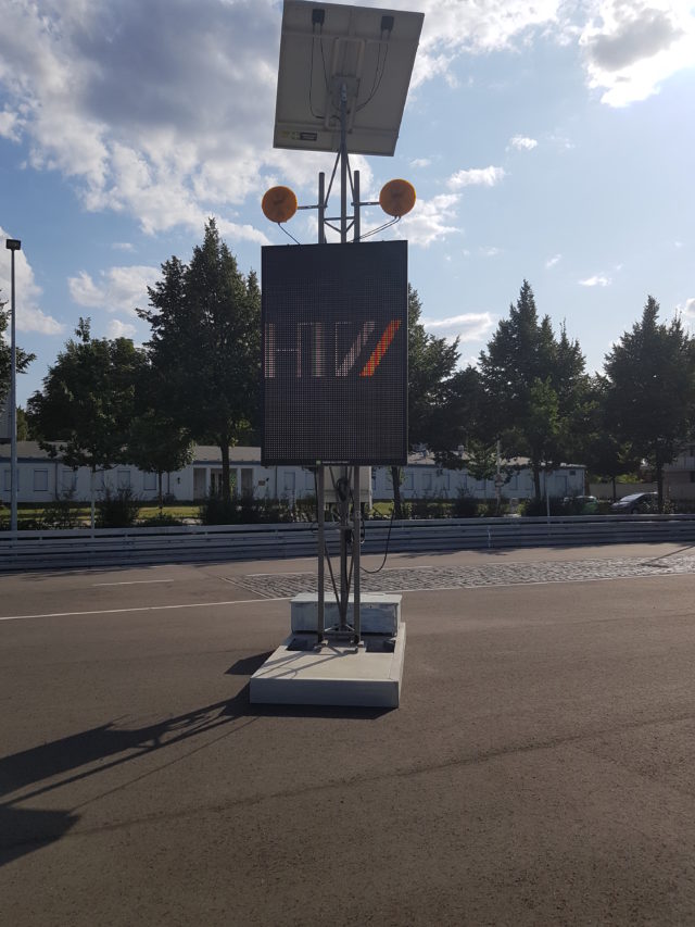
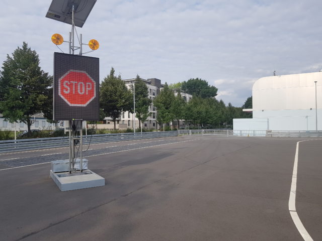
Auf dem Testfeld der HTW Dresden wurde für einen Zeitraum von einem Monat ein digitales Verkehrsschild durch die Firma Green Way Systems in Betrieb genommen. Für den Zeitraum von ca. einem Monat können darüber benutzerspezifische und standardisierte Verkehrssymbole eingeblendet werden.
 TTLab
TTLab
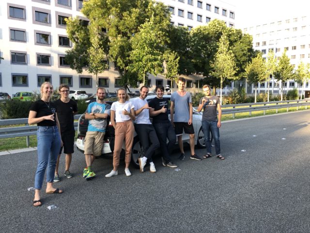
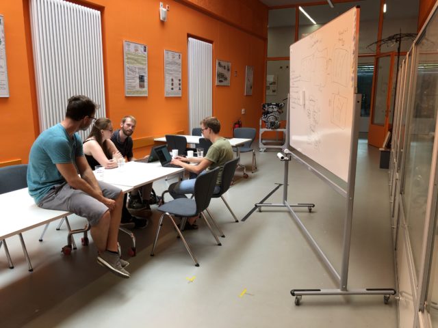
Saxony5-Hackathon – Tag 5
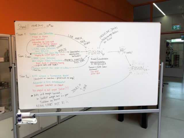
Tag 5 – das bedeutet Abschluss. Nach durchwachter Nacht konnten die Teilnehmer zwei Umsetzungen der Aufgabenstellung und mehrere ausbaufähige Alternativansätze präsentieren.

Nach den theoretischen Vorbetrachtungen ging es dann aufs Prüffeld zur großen Abschlussdemonstration. Dabei zeigte sich die Variante von Team #2 etwas robuster, hier gab es keine Probleme nach dem Richtungswechsel.
Danach ging es auf den Heimweg, nicht ohne vorher noch die Möglichkeiten zur Weiterarbeit zu diskutieren. Ihr dürft also auf Neuigkeiten gespannt sein…
Vielen Dank an dieser Stelle den Unternehmen für die Unterstützung.
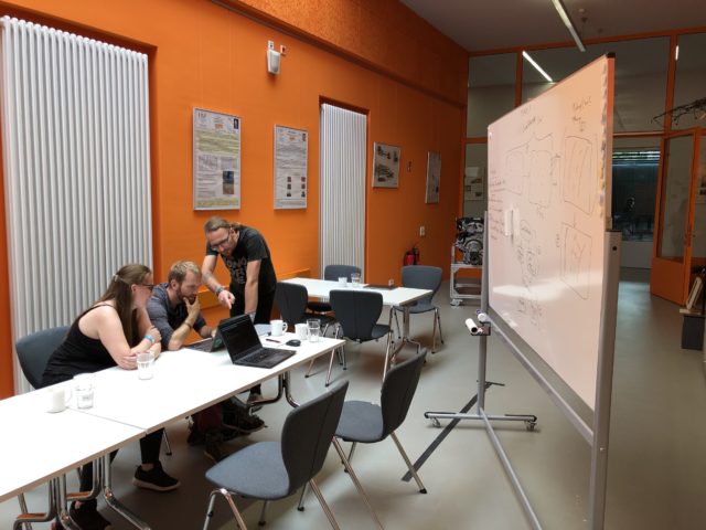
Saxony5-Hackathon – Tag 4
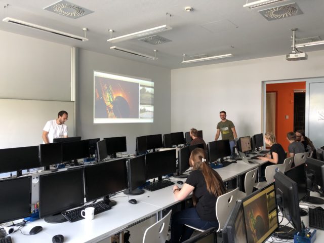
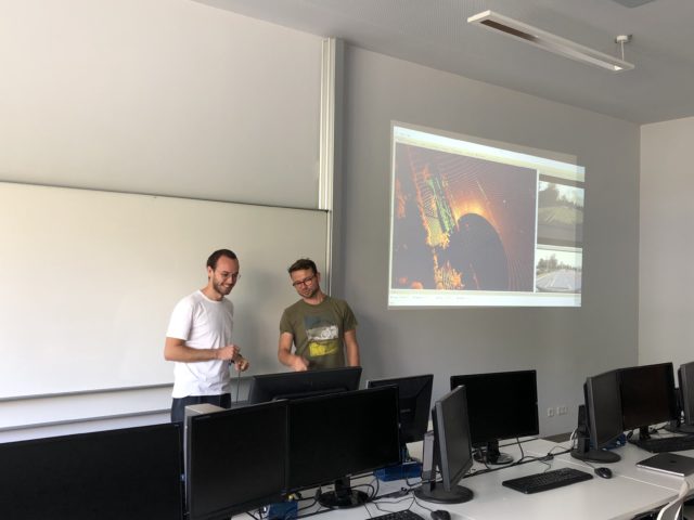
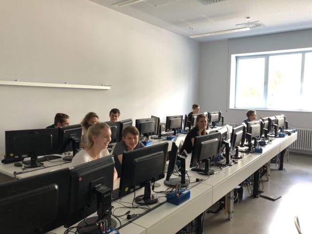
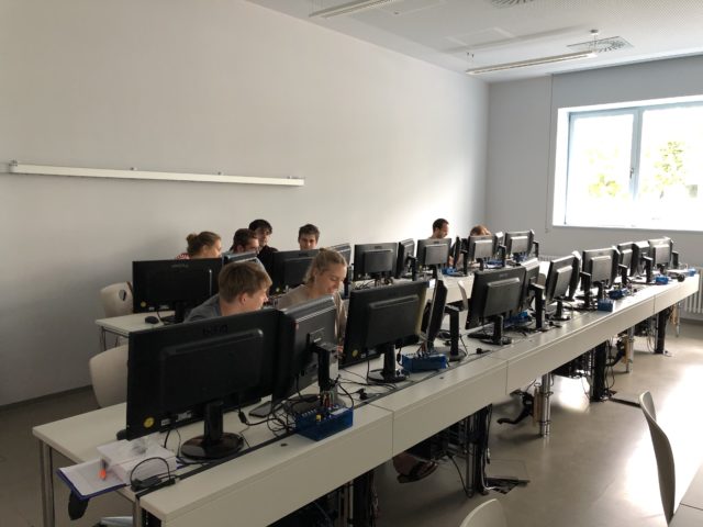
Wie jeden Tag der morgendliche Blick in den Rechnerpool. Fast könnte man meinen, die Gruppe hätte den Raum seit dem gestrigen Abend nicht verlassen. Doch wie der weitere Weg in den Flur zeigt, fand am Vorabend zu später Stunde noch eine Teambesprechung außerhalb des Rechnerpools statt.
Dank gemeinsamer Anstrengung und konsequenter Weiterarbeit konnte dann am Abend des heutigen Tages der erste Erfolg gefeiert werden. Zwar bleibt das Fahrzeug noch nicht ganz in der vorgesehenen Fahrspur, Lackschäden durch Touchieren der Leitplanke traten aber nicht auf. Das lässt für den letzten Tag hoffen.
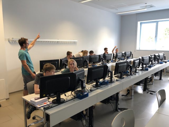
Saxony5-Hackathon – Tag 3
Der dritte Tag begann so, wie der zweite (an der HTW) endete – am Rechner. Erste Messungen wurden auch durchgeführt, das Ziel scheint also näher zu rücken.

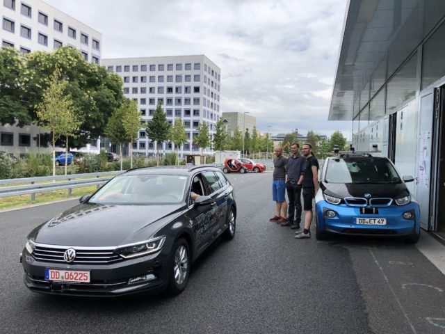
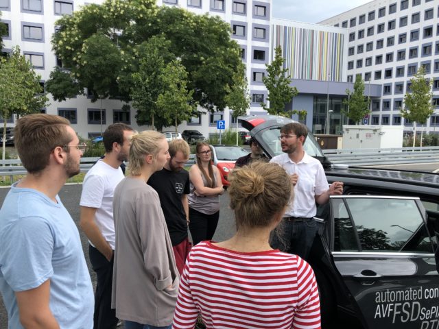
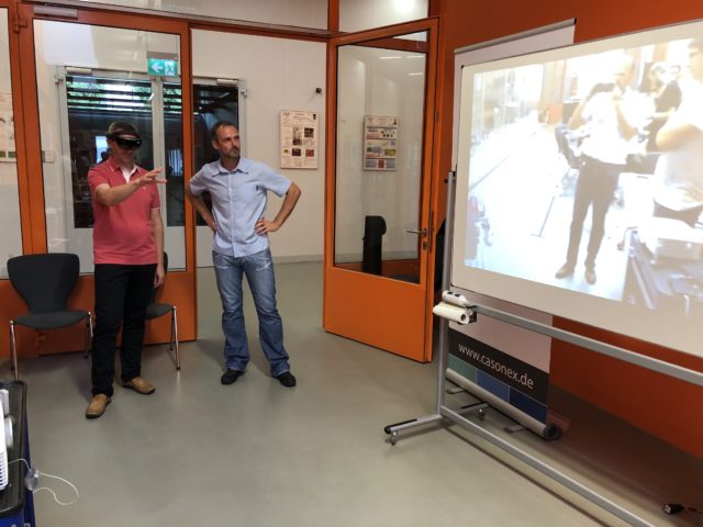
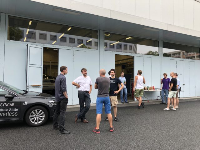
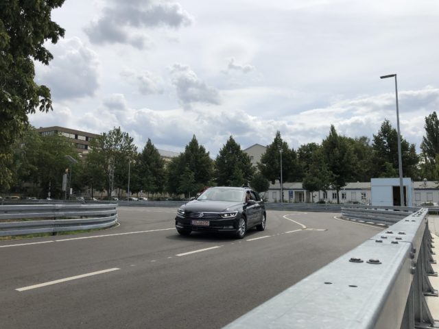
Am Nachmittag demonstrierte die FSD Fahrzeugsystemdaten GmbH aus Dresden dann ihren Versuchsträger für automatisierte Fahrfunktionen.
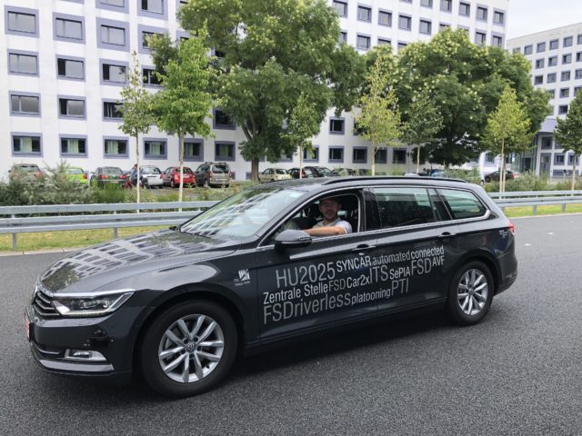
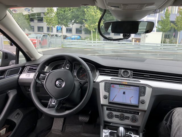
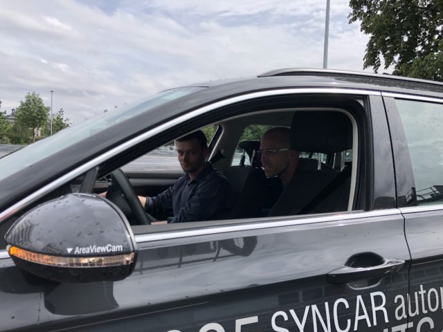

In den beiden folgenden Videos ist eine Messfahrt zu sehen.
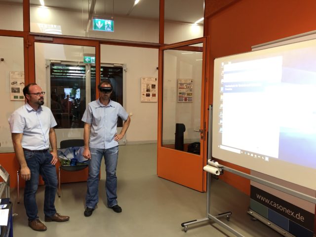
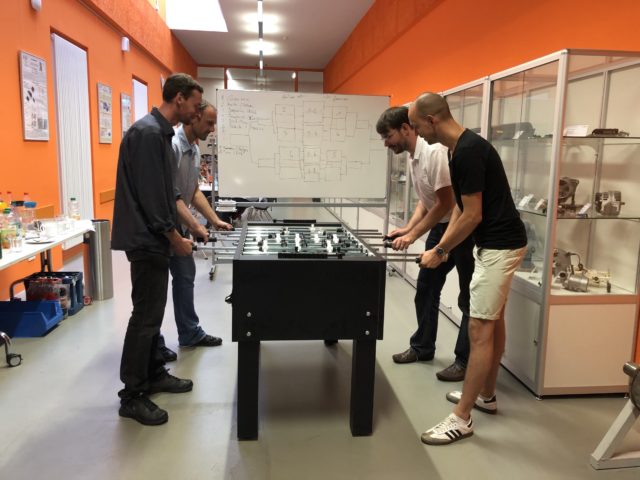
Nach dieser eindrucksvollen Demonstration erwartete die Studierenden ein Grillabend, der von der Firma Casonex mit interessanter Technik zur erweiterten Realität begleitet wurde.
Sieger im anschließenden Kickerturnier wurde das Mechlab-Team #1 (Glückwunsch und Dank an Dirk & Ecke), knapp gefolgt von den Champions der Casonex GmbH.
Saxony5-Hackathon – Tag 2
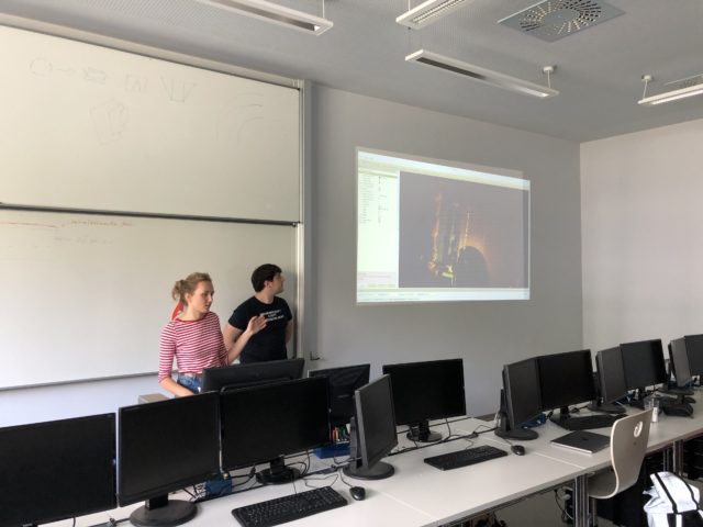
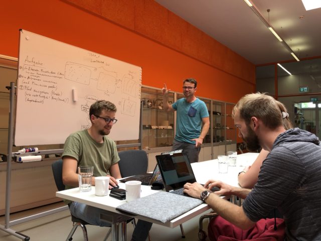
Der zweite Tag stand ganz im Zeichen der Funktionsentwicklung. Als erste Aufgabe wurde die Implementierung einer auf Lidardaten basierenden Spurführung ausgewählt, die Vorarbeiten dazu erfolgten bereits durch Christopher Dunkel (Blogbeitrag). Um die Dynamik zu erhöhen, treten zwei Teams gegeneinander an. Die nachfolgenden Bilder zeigen die intensive Programmierarbeit sowie die Unterstützung durch das Mechlab-Team. Dabei scheint es fast, dass es erste Nachahmer für Svens wilde Gesten gibt.
Erste Messungen fanden auch mit dem Passat der FSD Fahrzeugsystemdaten GmbH statt. Für Tag 3 ist hier eine Vorstellung der Automatisierung auf Basis einer dGPS-Ortung vorgesehen.
Saxony5-Hackathon – Tag 1
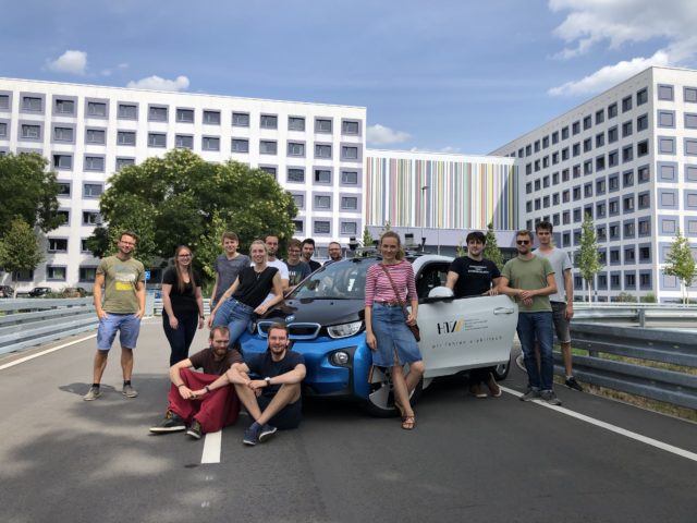
Am 05.08.2019 startete der 1. Hackathon zum Thema „Automatisierte Fahrfunktionen“. Insgesamt 11 Studierende der HTWK Leipzig und der HTW Dresden wollen neue Funktionen für ein Versuchsfahrzeug entwickeln.
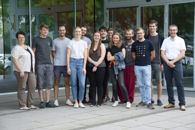
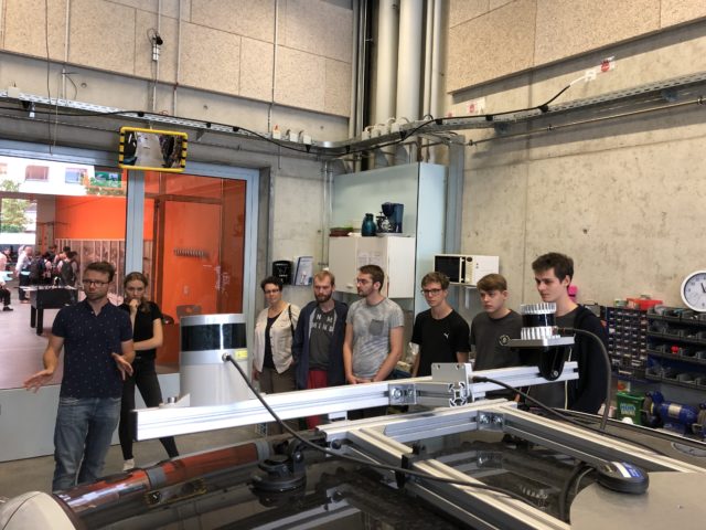
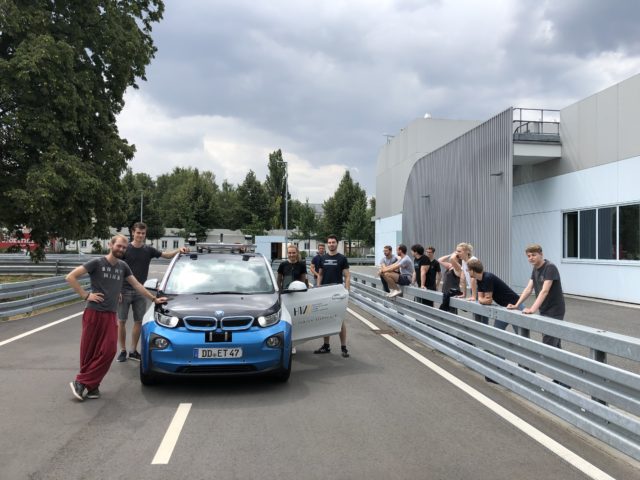
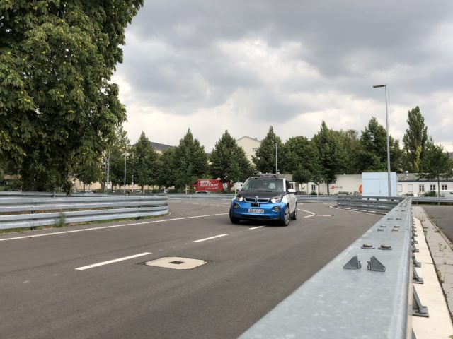
Der erste Tag stand im Zeichen der Vorstellung des Mechlab-Teams und der verfügbaren technischen Ausrüstung. Der aktuelle Stand im Versuchsträger BMW i3 wurde auf dem HTW-Prüffeld demonstriert. Die fachliche Betreuung wird von M. SC. Sven Eckelmann koordiniert.
Applying Filters on LiDAR Point Clouds

The Point Cloud Library (PCL) offers great possibilities for processing large point clouds. In the following article the principle of different filters and its application on pointclouds from Velodyne Puck and Ouster OS1 LiDARs using ROS shall be described.
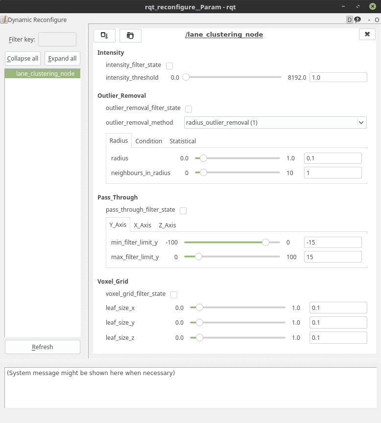
For quick configuration changes, all filter parameters can be changed via rqt dynamic reconfigure. So far 4 different types of filtration have been implemented:
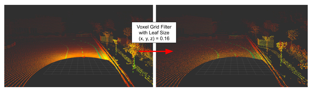
Voxel Grid
This type of filter allows downsampling of large point clouds (PCL Voxel Grid Filter). The parameter leaf_size describes the length of a box in 3 dimensions, in which all points are reduced to one point.
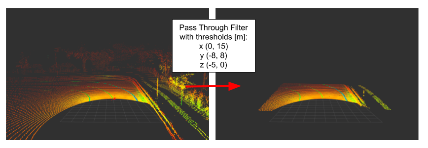
Pass Through
A pass through filter allows to restrict point clouds in their dimensions (PCL Pass Through Filter). The parameters are the min and max value of the points in meters, which should (not) be filtered.
Outlier Removal
The library offers different types of filters to remove noise and outliers.
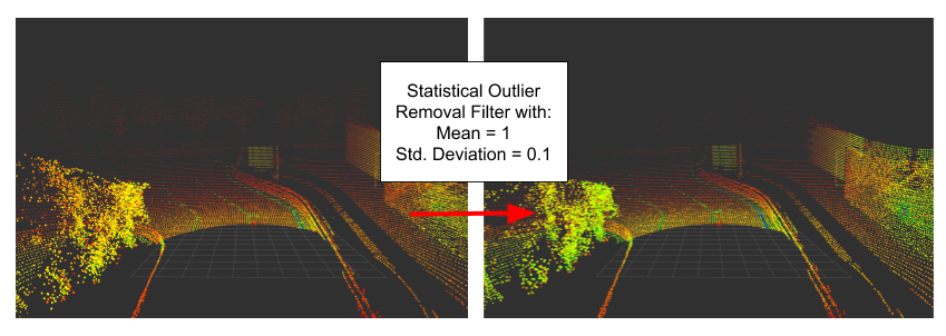
- Statistical Outlier Removal: The average distance from each point to its neighbours is calculated. Under the assumption that it is a gaussian distribution, a filtering can take place by using the parameters mean and standard deviation (PCL Statistical Outlier Removal Filter).
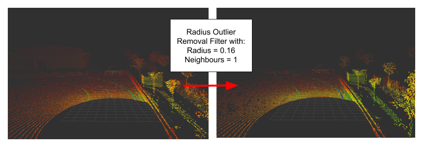
- Radius Outlier Removal: We define a certain number of points, which must be present within a radius (PCL Radius Outlier Removal Filter).
- Conditional Removal: The filtering object depends on the defined conditon. A condition could be described as a comparison between 2 thresholds. For example a point musst be musst be greater than and less than a given size (PCL Conditonal Outlier Removal Filter). It’s functionality can be compared to the Pass Through Filter.

Intensity Filter
The intensity filter is not part of PCL but the library in addition with Boost can be used to implement such a filter. A point in a cloud needs at least 3 informations (x, y, z) and optionally additonal an intensity or color informations. In our case we will define the PCL point type pcl::PointXYZI. Now a PCL point cloud pointer with the specified point type can be created as a typedef:
typedef typename pcl::PointCloud::Ptr PointCloudPtrWith Boost it’s easy to iterate through a sequence. Each point is assigned an intensity, which is compared afterwards:
BOOST_FOREACH (const pcl::PointXYZI &pt, input_cloud->points) {
    if (pt.intensity > intensity_threshold)) {
    output_cloud->points.push_back(PointXYZI_(pt.x,pt.y,pt.z,pt.intensity));
    }
}
PointXYZI_ is a inline helper function because the PCL library does not provide a PointXYZI constructor for all needed fields (x, y, z, intensity). Now the whole filter can be implemented as a class method:
PointCloudPtr
LaneClustering::intensityFilter (PointCloudPtr input_cloud, double& intensity_threshold)
{
    PointCloudPtr output_cloud (new pcl::PointCloud());
    BOOST_FOREACH (const pcl::PointXYZI& pt, input_cloud->points) {
        if (pt.intensity > intensity_threshold) {
            output_cloud->points.push_back(PointXYZI_(pt.x,pt.y,pt.z,pt.intensity));
        }
    }

    return (output_cloud);
}
The following image shows the application of the filter with different intensity thresholds to a point cloud of an Ouster OS1 lidar with 64 layers:
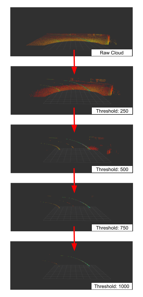
It is easy to see that many parts of the point cloud are filtered even at a very low limit value. From a value above 750 almost all points except the road markings are removed. If the limit value is further increased, parts of the track marking are also omitted and only the part with a retro-reflective marking remains.
The following videos show the application of all filters on point clouds from a Velodyne Puck and an Ouster OS1 lidar.
Patentanmeldung für Scheinwerfer-Prüfverfahren
Aufbauend auf Vorarbeiten zu neuen Methoden der Scheinwerferprüfung (siehe z.B. Diplomarbeit André Najort) wurden neue Konzepte für praxisnahe Verfahren entwickelt. Das nachfolgende Expose zeigt eine Kurzfassung der Methodik sowie den Verweis auf die Patentanmeldung. Bei Interesse kontaktieren sie uns bitte unter trautmann@htw-dresden.de.
Mechlab @ Cooper University NYC
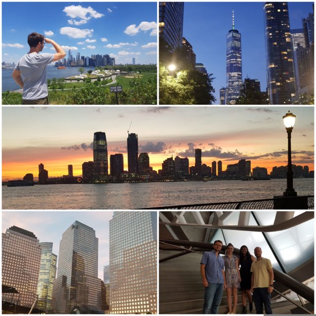
Cooper University NYC
Im Rahmen von NIVES bestand die Möglichkeit, unsere Aktivitäten mit der Cooper University in New York zu diskutieren und zukünftige gemeinsame Projekte zu besprechen. Als Ziel wurde die Entwicklung eines Mobilitätskonzeptes vereinbart, welches über den gemeinsamen Austausch von Studenten und Lehrkräften beider Hochschulen bearbeitet werden soll. Im Hinblick der Automatisierung wurden Testfelder in NYC, wie beispielsweise Gouverment Island besichtigt.
Untersuchung von neuen Fahrspurmarkierungen
Am 26.04.2019 starteten die Tests der retroreflektierenden und kontrastverstärkten Fahrspurmarkierungen der Firma 3M im 2-Wochen Rhythmus. Zuerst werden Messungen der ungereinigten Markierung mit einem Laserscanner durchgeführt. Nach einer Reinigung mit der bereitgestellten Kehrmaschine aus dem Projekt EBALD wird eine weitere Messung durchgeführt. Außerdem gab es bisher eine Vergleichsmessung unter leichtem Regen als Zusatzmessung.
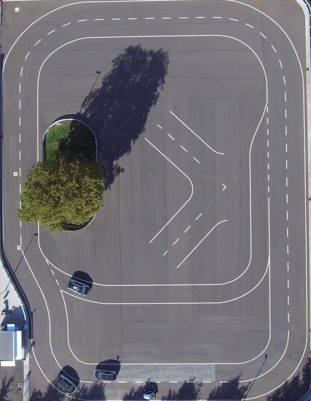
Bild 1: Testfeld Ansicht von oben 
Bild 2: 1. Messung
Die Farbe spiegelt die Intensität der Datenpunkte des Laserscanners dar, von blau für weniger intensiv bis orange für intensiver. Das Koordinatensystem ist auf dem Testfeld angelegt. Die Positionierung über die die gewonnen Laserdaten aufgetragen werden erfolgt über eine Sensordatenfusion mit extended Kalman-Filter. Daher kommen auch Ungenauigkeiten in der Transformation der Punkte auf das Testfeld. Die verbesserte äußere Fahrspur ist im Vergleich zur inneren deutlich gelber zu erkennen. Die zweite blaue Punktlinie am äußeren Rand stammt von den Banden rund um das Prüffeld (2).
Untersuchte Einflüsse
Verschmutzung
Im Laufe des Frühlings kam es vor allem zu starken Blütenanlagerungen durch die Bäume auf und in der Nähe der Markierungen (5-8). Dabei ist besonders anzumerken, dass durch die Anrauhung eine erhöhte Verschmutzung auf den neuen Markierungen festzustellen ist. Auch wenn hier die Schrägung des Testfeldes berücksichtigt werden sollte, die den Effekt verstärkt. Die Säuberung wird mit einer einmaligen Fahrt vorgenommen, um nicht zu sehr von Realbedingungen abzuweichen. Beide Markierungen können gleich gut gereinigt werden.
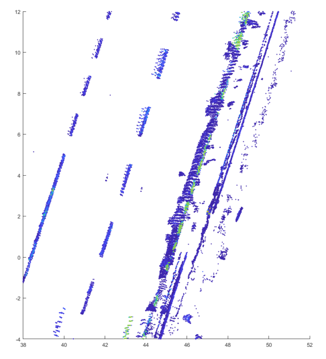
Bild 3: Laserdaten vor Reinigung 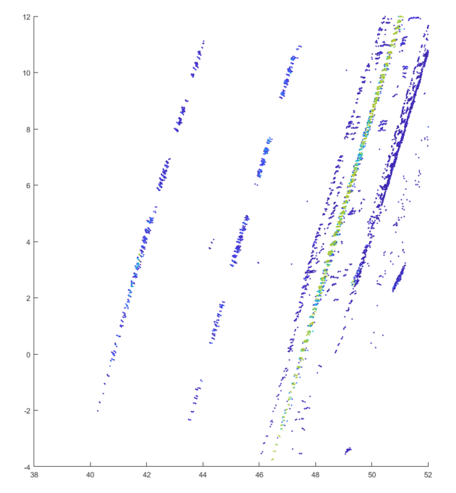
Bild 4: Laserdaten nach Reinigung 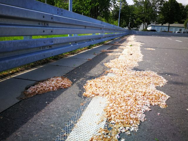
Bild 5: Sehr starke Blütenverschmutzung 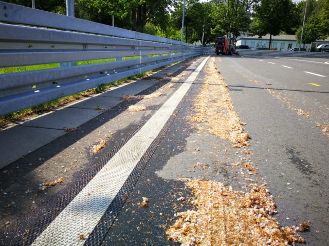
Bild 6: Fahrspurmarkierung nach Reinigung

Bild 7: Leichte Verschmutzung 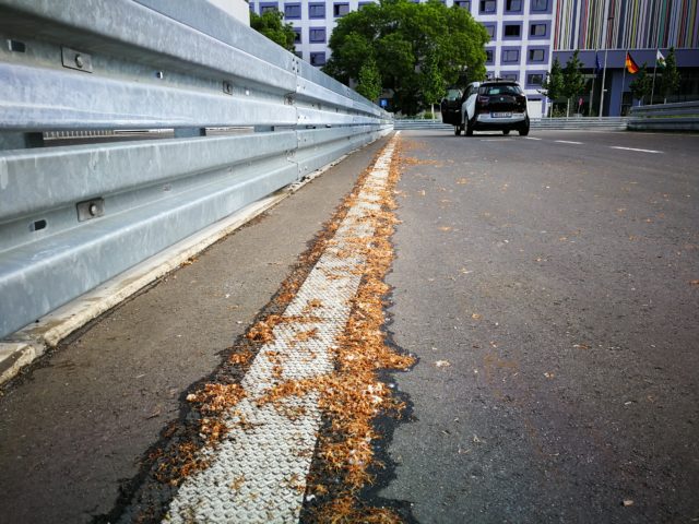
Bild 8: Fahrspurmarkierung nach Reinigung 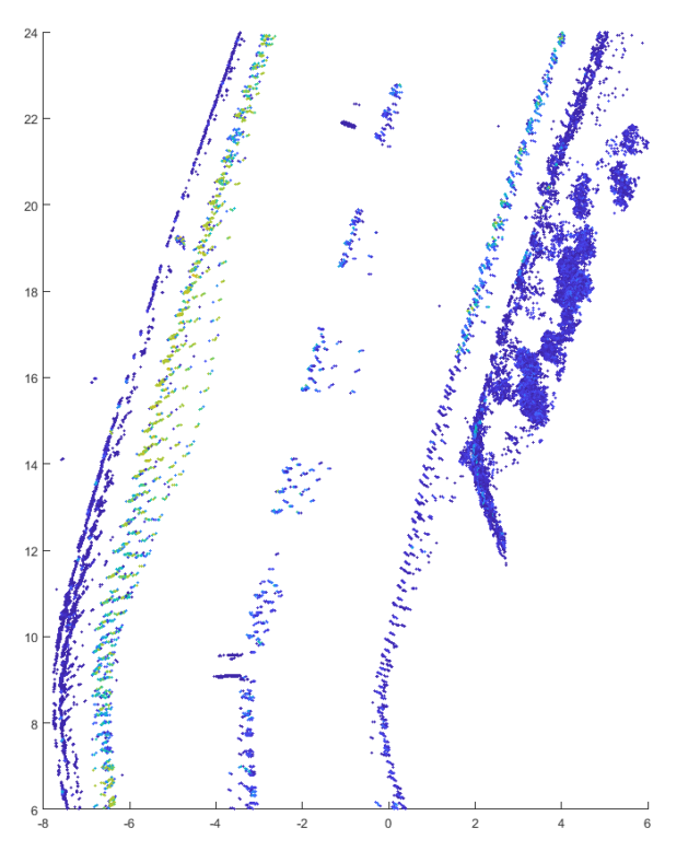
Bild 9: Laserdaten nach Reinigung 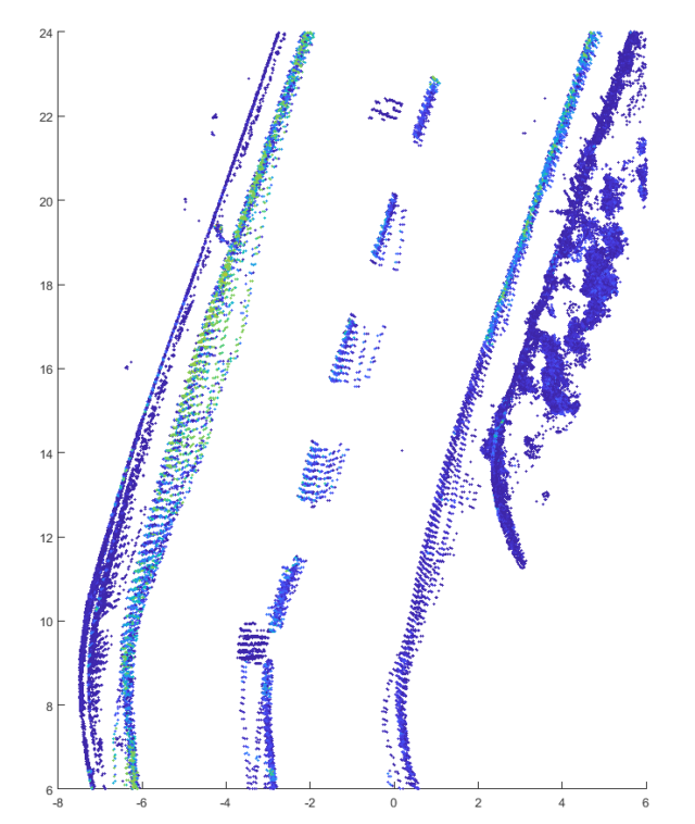
Bild 10: Laserdaten vor Reinigung
Bei der vollständigen Überdeckung ist die Intensität logischerweise stark verringert (3), außerdem sind die Punkte zerstreut. Nach der Reinigung stellt sich der Normalzustand ein (4). Bei der leichten Verschmutzung sind die gleichen Effekte, allerdings in deutlich geringerem Ausmaß, zu beobachten (10). Trotz der stärkeren Verschmutzung liefert hier die neue Markierung immer noch bessere Daten als die herkömmliche.
Regen
Der Einfluss durch Regen ist die größte Stärke im Vergleich zu herkömmlichen Fahrspurmarkierungen.
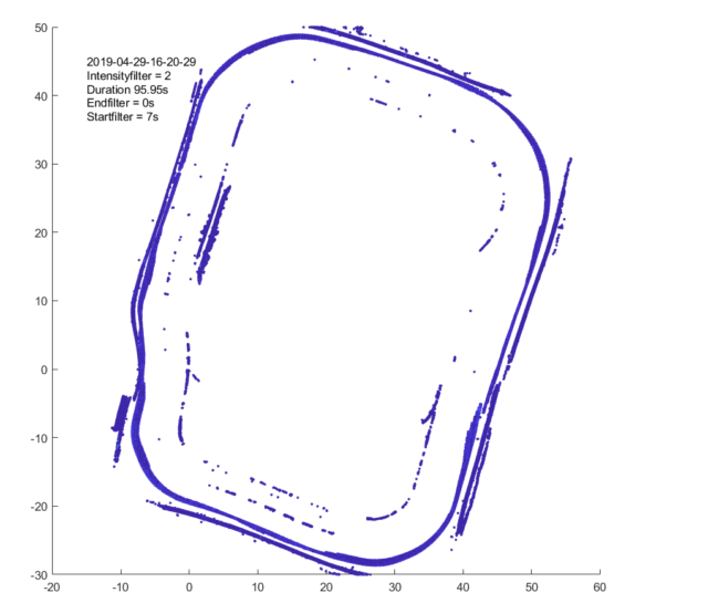
Bild 11: Regenmessung 29.04.19 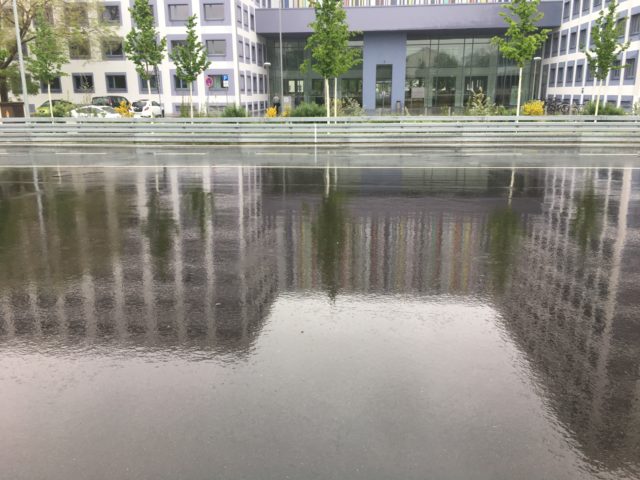
Bild 12: Regenmessung 29.04.19 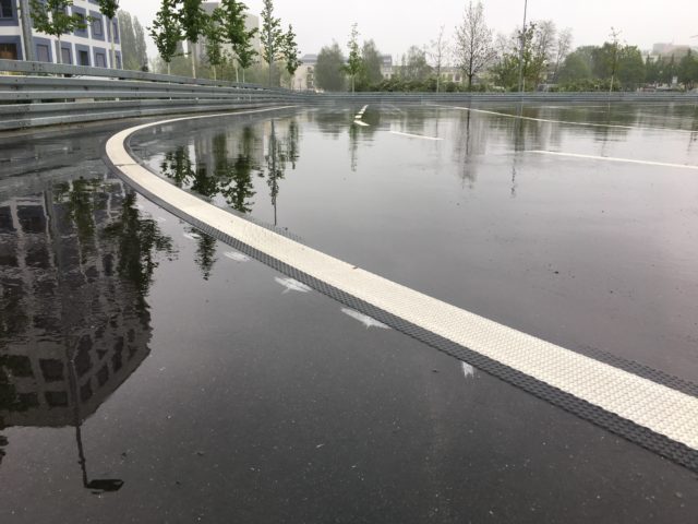
Bild 13: Regenmessung 29.04.19
Im Bild ist deutlich zu sehen, dass trotz eines verringerten Intensitätsfilters bei leichter Feuchte die innere Markierung kaum zu sehen ist (11). Auch die Intensität der speziellen Markierung ist verringert, aber noch deutlich auszumachen. Hierbei bewältigt die neue Fahrspurtechnologie das Problem von Lidar mit feuchter Straße sehr gut.
Beschädigung
Der bis jetzt am geringsten zu spürende Einfluss, ist die Verminderung der Reflektivität durch die regelmäßige Belastung auf die Markierungen durch die Metallborsten der Kehrmaschine. Nach 4 Reinigungen ist kein Unterschied zu erkennen. (Vgl. 14 und 15)
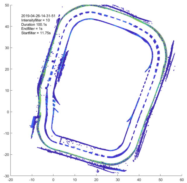
Bild 14: 1. Messung ungereinigt 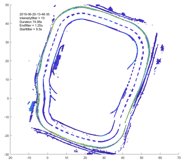
Bild 15: 5. Messung, 4 Reinigungen später
Allerdings kam es bereits zu leichten Ablösungen und Fadenziehen an den Übergangsstellen. (16-20)
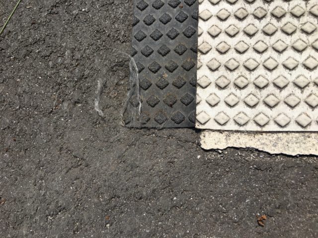
Bild 16 
Bild 17 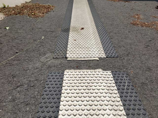
Bild 18 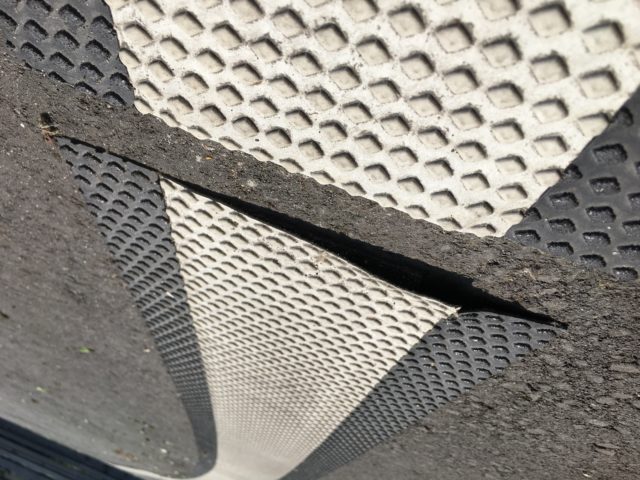
Bild 19 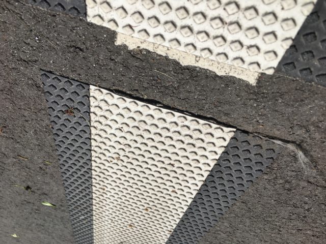
Bild 20
Hierbei ist anzumerken, dass die Anbringung der Markierungen nicht ideal erfolgte. Sie wurden mit nicht optimalem Kleber über den herkömmlichen Markierungen angebracht, wie es normalerweise nicht vorgesehen ist.
Bisheriges Fazit
Die retroreflektierenden Fahrspurmarkierungen erfüllen ihren Zweck gut und halten den Belastungen im Allgemeinen stand. Sie verbessern die wahrgenommene Intensität durch Lidar deutlich. Allerdings sind die Probleme mit dem bisherigen Einzelfall der sehr starken Verschmutzung und der Beschädigung weiter im Auge zu behalten.
Nach der Testphase auf dem Prüffeld werden die Tests auf der B170 fortgesetzt.