The prediction of steering angles for a vehicle depending on its environment is a general problem for which some approaches already exist. The classic approach is based on the recognition and tracking of lanes with the aid of image processing. With this method, the images are captured, processed and the detected lanes are then represented by polynomials, on the basis of which the necessary steering angle is calculated. Another way to determine the steering angle based on the environment of the vehicle is to use a neural network. According to the Nvidia paper (https://arxiv.org/pdf/1604.07316v1.pdf), this approach shall be examined in the following.
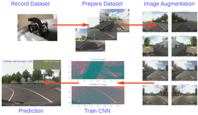
The aim is to design a neural network and to train it with data from the laboratory test track in order to be able to make predictions regarding the necessary steering angle. So the first step is to record as much data (as possible) from the track.
1. Generate the Dataset
Only 2 informations are important: Images of the track out of the position of the vehicle and the corresponding steering angle at the time of recording. In the best case there are several images from different positions available but in our case we only use a centrally positioned Raspberry Pi camera at first. After driving 5 laps in one direction you should drive another 5 laps in the other direction to help the neural network to generalise. The test vehicle for the measurements is a modified Renault Twizy, which is currently used in the project Platooning (http://www.htw-mechlab.de/index.php/forschung/platooning/projektfortschritt-timeline/). Camera frames and steering angles are merged, processed and stored via a ROS node. In parallel, pandas creates a CSV file containing the names of the camera frames and the corresponding steering angle.
After this process, a dataset should be created whose length depends on the recording time. For this example about 10.000 images were taken. The following lines represent 7 random lines from this dataset:
       timestamp         filename  steering_angle
2440  243.939088  frame002440.jpg        0.007333
7036  703.538947  frame007036.jpg       -0.226222
6922  692.139068  frame006922.jpg        0.012889
8715  871.439109  frame008715.jpg       -0.223333
5700  569.939100  frame005700.jpg       -0.033333
6960  695.939064  frame006960.jpg       -0.182222
8326  832.539025  frame008326.jpg        0.010667
2. Prepare the Dataset
The next step contains preparing the data. For this it is helpful to plot the distribution of steering angles from recorded data:
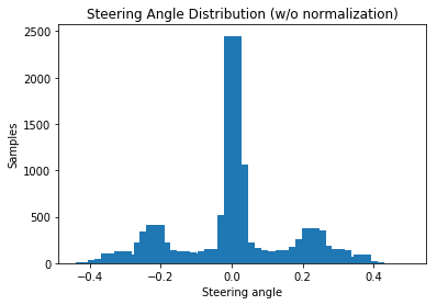
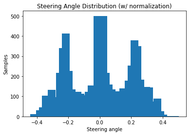
It can be seen that considerably more steering angles were recorded in the 0 degree range. This also makes sense, because the test track consists mainly of straight tracks. For the model, this is problematic, because the car is biased to drive straight all the time. One solution could be to record more data just from curves. This results automatically in a larger dataset, which is to be examined later. For now, it’s easier to reduce the datatset with redundant steering angles. Additionally the data of the turning maneuver for the direction change can be removed here. The normalized steering angle distribution (with about 7.000 remaining images) now look like this:
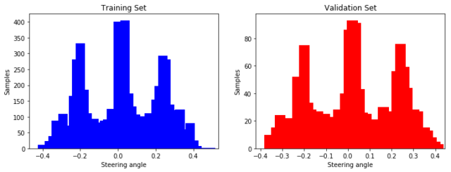
3. Split the Datatset
In the next step the dataset can be split into a training dataset, a validation datatset and optionally a test datatset. The training datatset is the largest part and is used to train the model. The neural network learns from this dataset and updates its weights and biases. The validation dataset is used to tune the hyperparameters (e.g. learning rate and number of hidden units) of the network with new images to avoid overfitting (occurs when the capacity of a network is to high and the model can not be generalised).
After training the network sucessfully the test dataset can be used to determine what predictions the network makes for new data. This part is not necessary because the network is to be tested directly with new measurement data on the test track and we therefore only need a division between training and validation:
4. Augment the Dataset
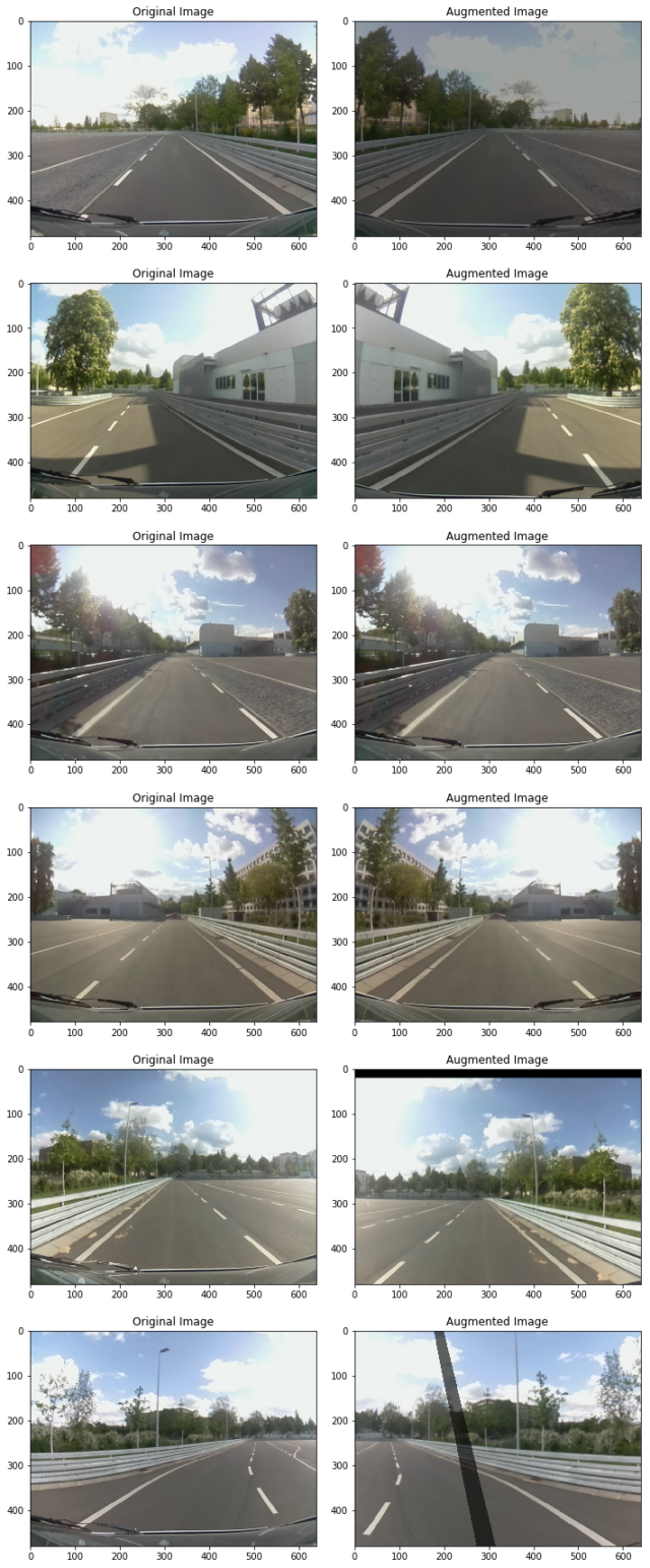
In order to counteract the fact of the small number of data, new data is to be generated in the following by image augmentation. During this process we create new data by modifying the existing dataset for our model to use by the training process. For now we will use 5 different augmentation techniques:
- random shadow
- random brightness
- random flipping
- random zooming
- random shifting
The following plot shows 6 random images with a corresponding augmentation technique:
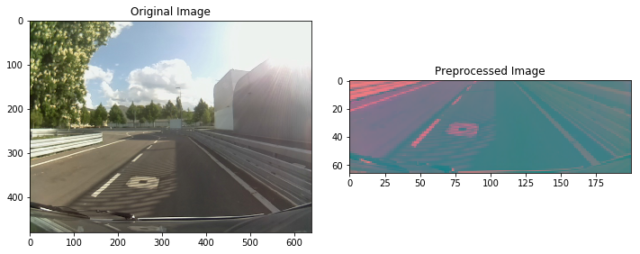
5. Preprocess the Images
Now its time to edit the images so that they can be processed by the network. At first we need to determine a region of interest (ROI). This region should contain all the informations which are necessary for the steering angle prediction (e.g the lanes). Afterwards we change the colorspace from RGB to YUV, resize the image according to the input size of the network (200×66) and apply a Gaussian blur:
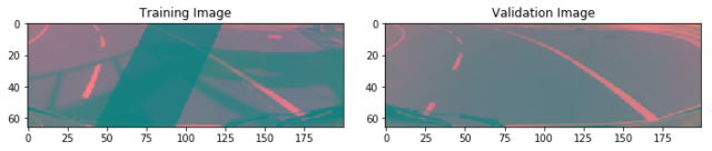
6. Generate Batches
The last step before generating and training our model is the creation of a batch generator. The batch generator is used to generate a defined number of preprocessed images with associated labels from the input data. The number of samples that will be fed during one forward/backward pass trough the network is called batch size. The following figure shows a training and validation image randomly generated by the generator:
7. Create the Model
As mentioned above we will use a popular architecture from Nvidia to create the model. This type of model consists of several Convolutional Layers (CNN) followed by several Fully Connected Layers (Dense). Convolutional Neural Networks (CNNs) are commonly used to analyse images. They consists of Input Layers, Convolutional Layers, Pooling Layers, Fully Connected Layers and Output Layers.
- Convolutional Layers extract and learn specific image features which can be used to help classify the image
- Pooling Layers helps avoid overfitting during reducing the dimensionality of representation of each feature map
- Fully Connected Layers are built the same way as a normal Neural Network
With Keras (and TensorFlow as backend) we don’t have to care about input and output sizes of hidden layers in the network Just the input dimension from the first layer has to be equal to the image dimension and all further layers will get its size automatically. The full implementation of the Nvidia model and Keras looks like this:
def nvidia_model():
  # Input Layer
  model = Sequential()

  # Convolutional Layers
  model.add(Conv2D(24, (5, 5), strides=(2, 2), input_shape=(66, 200, 3), activation='elu'))
  model.add(Conv2D(36, (5, 5), strides=(2, 2), activation='elu'))
  model.add(Conv2D(48, (5, 5), strides=(2, 2), activation='elu'))
  model.add(Conv2D(64, (3, 3), activation='elu'))
  model.add(Conv2D(64, (3, 3), activation='elu'))

  # Flatten Layer
  model.add(Flatten())

  # Dense Layers
  model.add(Dense(100, activation='elu'))
  model.add(Dense(50, activation='elu'))
  model.add(Dense(10, activation='elu'))

  # Output Layer
  model.add(Dense(1))

  optimizer = Adam(lr=1e-4)
  model.compile(loss='mse', optimizer=optimizer)
  return model
8. Train the Model
Before the model is trained, it is helpful to get a summary of the model and the generated layers:
Layer (type)                 Output Shape              Param #
=================================================================
conv2d_6 (Conv2D)            (None, 31, 98, 24)        1824
_________________________________________________________________
conv2d_7 (Conv2D)            (None, 14, 47, 36)        21636
_________________________________________________________________
conv2d_8 (Conv2D)            (None, 5, 22, 48)         43248
_________________________________________________________________
conv2d_9 (Conv2D)            (None, 3, 20, 64)         27712
_________________________________________________________________
conv2d_10 (Conv2D)           (None, 1, 18, 64)         36928
_________________________________________________________________
flatten_2 (Flatten)          (None, 1152)              0
_________________________________________________________________
dense_5 (Dense)              (None, 100)               115300
_________________________________________________________________
dense_6 (Dense)              (None, 50)                5050
_________________________________________________________________
dense_7 (Dense)              (None, 10)                510
_________________________________________________________________
dense_8 (Dense)              (None, 1)                 11
=================================================================
Total params: 252,219
Trainable params: 252,219
Non-trainable params: 0
_________________________________________________________________
None
The generated model consists of about 250.000 parameters and 27 million connections, which is a pretty amazing size! Now the model can be fed with our data and other parameters like batch size and epochs. For all those of you who did not have several Nvidia K80 GPUs at home there is a free cloud-based alternative called: Google Colab! Colab is a machine learning research tool with GPU acceleration for the browser based on Jupyter notebooks (https://colab.research.google.com/).
The training process takes about one hour. During that process it can be tracked how loss and validation loss changes and afterwards we can plot the data:
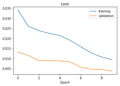
The generated model can now be downloaded and implmented in the ROS steering prediction node.
9. Predict Steering Angles
Predicting steering angles follows the same procedure as described during the dataset generation, but without the need to record the data. We capture camera frames, preprocess them as described in chapter 5 and feed them into the model, which predicts a steering angle between -1 and +1. The result is shown in the following video.
10. Improvements
The result is not bad, but in the next step the following improvements will be implemented:
- Install more cameras to record larger datasets and capture a steering angle from different positions.
- Refine the ROI, in particular the peripheral areas.
- Enlarge the dataset which contains curves.
- Optimize the model parameters (activation function, batch size, epochs, …).
- Improve and add more augmentation functions.